Amazon Athena Cost Optimization: Partition Pruning, Compression, and Iceberg Tables
Quick summary: Athena still bills ~$5/TB scanned (or Capacity Reservations by DPU). July 2026 refresh — partitions, Parquet/Iceberg, workgroups, and when provisioned capacity wins.
Key Takeaways
- Athena still bills ~$5/TB scanned (or Capacity Reservations by DPU)
- July 2026 refresh — partitions, Parquet/Iceberg, workgroups, and when provisioned capacity wins
- Amazon Athena stays cheap when layout is right
- As of July 2026, default billing is still per TB scanned (commonly ~$5/TB — verify pricing), with a 10 MB minimum; you can also buy Capacity Reservations (DPU-hour) for concurrency SLAs
- Engagement shape (anonymized): SaaS product analytics lake, ~80 GB/day Parquet events, ~2k Athena queries/day across three workgroups
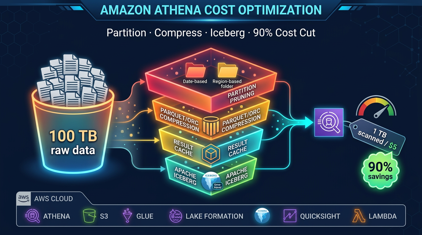
Table of Contents
Amazon Athena stays cheap when layout is right. As of July 2026, default billing is still per TB scanned (commonly ~$5/TB — verify pricing), with a 10 MB minimum; you can also buy Capacity Reservations (DPU-hour) for concurrency SLAs. Same SQL, wrong layout → multi-dollar scans; Parquet + partitions + Iceberg skipping → cents.
Engagement shape (anonymized): SaaS product analytics lake, ~80 GB/day Parquet events, ~2k Athena queries/day across three workgroups. After Iceberg + workgroup scan caps, top-20 queries dropped from multi-GB scans to tens of MB (directional; your selectivity differs).
Reproduce this: Athena scan checklist · Iceberg compaction worksheet
The Athena Cost Equation
Every dollar you spend on Athena is directly proportional to bytes scanned. The optimization problem therefore reduces to a single question: how do you prevent Athena from reading data it does not need?
There are four mechanisms Athena uses to skip data:
- Partition pruning — skip entire S3 prefixes based on partition columns in your WHERE clause
- Column pruning — read only the columns in your SELECT (requires columnar format)
- Row group statistics — skip blocks of rows within a file (requires Parquet/ORC)
- Iceberg data skipping — skip entire files based on manifest-level min/max column statistics
Stack all four, and a query that previously scanned 1 TB might scan 10 GB. That is a 99% cost reduction with zero change to query logic.
Partitioning: The Biggest Single Lever
Partitioning organizes your S3 data into prefixes that correspond to column values. Athena reads the partition metadata from the Glue Data Catalog and uses it to construct a list of S3 prefixes to scan. Any partition whose prefix does not match your WHERE clause is excluded entirely — Athena never issues an S3 GET for those files.
Hive-Style Partitioning
The standard pattern is Hive-style key-value prefixes:
s3://my-datalake/events/
  year=2026/month=04/day=18/
    part-00001.parquet
    part-00002.parquet
  year=2026/month=04/day=17/
    part-00001.parquet
A query with WHERE year = 2026 AND month = 04 AND day = 18 scans only the year=2026/month=04/day=18/ prefix. A year of daily data has 365 partitions — daily filtering means Athena reads 1/365th of the total data.
Define partitions in your CREATE TABLE statement:
CREATE EXTERNAL TABLE events (
    event_id STRING,
    user_id  STRING,
    event_type STRING,
    payload  STRING,
    event_ts TIMESTAMP
)
PARTITIONED BY (year INT, month INT, day INT)
STORED AS PARQUET
LOCATION 's3://my-datalake/events/'
TBLPROPERTIES ('parquet.compress'='ZSTD');
Partition Discovery
After adding new data to S3, Athena needs to know the new partitions exist. Three approaches:
MSCK REPAIR TABLE: Scans all S3 prefixes under the table location and registers any new partitions it finds. Simple but slow for large numbers of partitions. Avoid for tables with thousands of partitions.
ALTER TABLE ADD PARTITION: Explicitly adds a partition in a single DDL statement. Fast and precise — good for scheduled pipelines where you know the exact new partition.
Partition Projection: Virtual partitions defined entirely in table properties without any Glue Catalog entries. Athena generates the partition list from a mathematical formula (date ranges, integer ranges, enumerated values) rather than Catalog lookups. Eliminates Catalog overhead completely. Best for date-partitioned tables with predictable ranges.
-- Partition projection example for a date-partitioned table
CREATE EXTERNAL TABLE events (...)
PARTITIONED BY (event_date STRING)
...
TBLPROPERTIES (
  'projection.enabled' = 'true',
  'projection.event_date.type' = 'date',
  'projection.event_date.range' = '2024-01-01,NOW',
  'projection.event_date.format' = 'yyyy-MM-dd',
  'storage.location.template' = 's3://my-datalake/events/${event_date}/'
);
With projection enabled, a query with WHERE event_date = '2026-04-18' resolves the S3 prefix mathematically without any Catalog API call. For tables with 1,000+ partitions, partition projection can eliminate seconds of overhead per query.
Choosing Partition Keys
The right partition key matches your most common query filters. Common patterns:
- Event logs: partition by
year/month/dayordate— most queries filter to recent days or specific date ranges - User data: partition by
regionortenant_id— queries typically filter to a specific tenant or geography - Transaction data: partition by
year/month— financial queries rarely span more than a month without aggregation
Over-partitioning is a real problem. If you partition by hour and write 100 files per hour for a year, you have 876,000 S3 prefixes. Athena’s LIST operations to discover partitions become a bottleneck. A rule of thumb: each partition should contain files totaling at least 128 MB of data. If your hourly data is only 5 MB, partition by day instead.
Columnar Formats: Parquet vs ORC vs CSV
Why Columnar Formats Matter
Row-based formats (CSV, JSON, TSV) store records row by row. To read column A from a million-row table, Athena must read all bytes of every row — including columns B, C, D, and E that you never asked for.
Columnar formats (Parquet, ORC) store data column by column. A query SELECT revenue FROM orders WHERE customer_id = 'C001' reads only the revenue and customer_id columns. If your table has 50 columns and your query touches 3, columnar format gives you roughly a 16x reduction in bytes read before compression.
Parquet vs ORC
Both Parquet and ORC are excellent choices. Parquet is more widely adopted in the AWS ecosystem (Glue, Athena, EMR, Redshift Spectrum, Amazon Data Firehose all support it natively). ORC has marginally better predicate pushdown in some scenarios. For greenfield projects, use Parquet.
Compression: Snappy vs Zstd
Parquet supports multiple compression codecs per row group. The two most relevant for Athena:
Snappy: Fast compression and decompression. Lower CPU overhead but lower compression ratio (~2x for typical log data). Good choice when CPU is your bottleneck.
Zstd (Zstandard): Higher compression ratio than Snappy (~3-4x for typical log data) with still-reasonable decompression speed. Athena supports Zstd natively. For cost optimization, Zstd is the better choice — you pay per byte scanned, so smaller files directly reduce your bill. Use parquet.compress = ZSTD in your table properties.
Converting CSV to Parquet
If you have existing CSV data in S3, a one-time AWS Glue job converts it to partitioned Parquet. A simple PySpark script:
from awsglue.context import GlueContext
from pyspark.context import SparkContext

sc = SparkContext()
glc = GlueContext(sc)

# Read raw CSV
df = glc.create_dynamic_frame.from_catalog(
    database="raw",
    table_name="events_csv"
).toDF()

# Write as Parquet with Zstd compression, partitioned by date
df.write \
    .mode("overwrite") \
    .option("compression", "zstd") \
    .partitionBy("year", "month", "day") \
    .parquet("s3://my-datalake/events-parquet/")
Run this once as a Glue job, then switch future ingestion to write Parquet directly (Amazon Data Firehose supports Parquet output natively via its data format conversion feature).
File Size Optimization
File size is a frequently overlooked performance and cost factor. Athena parallelizes query execution by splitting work across files. Too many small files create excessive overhead; too few large files limit parallelism.
Target file size: 128 MB to 1 GB per Parquet file.
The Small File Problem
Streaming ingestion pipelines (Amazon Data Firehose, Flink, Spark Streaming) write many small files. A Firehose stream buffering for 60 seconds at 1 MB/s produces a 60 MB file — still below optimal. At 100 KB/s, you get 6 MB files — far too small. For high-cardinality partition keys, the problem compounds: thousands of partitions each receiving trickle writes can produce millions of tiny files.
Fix 1: Tune Firehose buffer settings. Firehose lets you configure buffer size (1 MB to 128 MB) and buffer interval (60 to 900 seconds). For low-volume streams, set a 128 MB buffer with a 15-minute interval to allow file accumulation.
Fix 2: Periodic compaction. Schedule a nightly Glue job that reads all files written in the past day and rewrites them as fewer, larger Parquet files. This is often called “compaction” or “small file remediation.”
Iceberg Automatic Compaction
Apache Iceberg handles compaction natively via a SQL procedure:
CALL system.rewrite_data_files(
    table => 'db.events',
    strategy => 'binpack',
    options => map('target-file-size-bytes', '134217728')  -- 128 MB
)
This Athena procedure (available for Iceberg v2 tables) rewrites small files into target-sized files without downtime. Queries continue running against the table while compaction runs. Schedule it via AWS Glue or EventBridge + Lambda.
Apache Iceberg: Data Skipping Beyond Partitions
Partitioning prunes at the directory level. Iceberg adds file-level skipping via manifest metadata — a qualitatively different (and more powerful) optimization layer.
How Iceberg Metadata Works
Every Iceberg table has a metadata hierarchy:
Table Metadata JSON
  └── Snapshot
        └── Manifest List
              ├── Manifest File A (lower_bound: 2026-04-01, upper_bound: 2026-04-10)
              │     ├── data-file-001.parquet (min: 2026-04-01, max: 2026-04-03)
              │     └── data-file-002.parquet (min: 2026-04-04, max: 2026-04-07)
              └── Manifest File B (lower_bound: 2026-04-11, upper_bound: 2026-04-18)
                    ├── data-file-003.parquet (min: 2026-04-11, max: 2026-04-14)
                    └── data-file-004.parquet (min: 2026-04-15, max: 2026-04-18)
Each manifest file records the min and max value of every column for every data file it covers. When Athena evaluates WHERE event_date = '2026-04-05':
- Read manifest list — identifies which manifest files could contain
2026-04-05 - Read manifest A —
data-file-001has max2026-04-03(skip),data-file-002has range2026-04-04to2026-04-07(read) - Read manifest B — lower bound is
2026-04-11(skip entire manifest)
Result: Athena reads exactly one data file instead of all four. As data volume grows, this file-level skipping becomes increasingly valuable — especially for queries that filter on non-partition columns.
Creating Iceberg Tables in Athena
CREATE TABLE events_iceberg (
    event_id   STRING,
    user_id    STRING,
    event_type STRING,
    amount     DECIMAL(18,2),
    event_date DATE,
    created_at TIMESTAMP
)
LOCATION 's3://my-datalake/events-iceberg/'
TBLPROPERTIES (
    'table_type' = 'ICEBERG',
    'format' = 'parquet',
    'write_compression' = 'zstd',
    'optimize_rewrite_delete_file_threshold' = '10'
);
Athena supports Iceberg v2 table format. Iceberg v3 is not yet supported in Athena as of April 2026.
Partition Evolution
One of Iceberg’s most practical features for cost optimization is partition evolution. With Hive-style tables, changing the partitioning scheme requires rewriting all data and creating a new table. With Iceberg, you change the partition spec going forward — historical data retains the old partitioning, new data uses the new scheme, and queries transparently handle both.
-- Start with monthly partitioning
ALTER TABLE events_iceberg
ADD PARTITION FIELD months(event_date);

-- Later, switch to daily partitioning as data volume grows
ALTER TABLE events_iceberg
DROP PARTITION FIELD months(event_date);

ALTER TABLE events_iceberg
ADD PARTITION FIELD days(event_date);
Historical monthly partitions remain intact. New data is daily-partitioned. No rewrite required.
Iceberg ACID Operations: MERGE INTO for CDC Patterns
Hive-style Athena tables are append-only — you cannot update or delete individual rows. Iceberg tables support full ACID operations, enabling change data capture (CDC) patterns that are otherwise very difficult in a data lake.
MERGE INTO for Upserts
MERGE INTO events_iceberg AS target
USING staging_events AS source
ON target.event_id = source.event_id
WHEN MATCHED AND source.updated_at > target.updated_at THEN
    UPDATE SET
        event_type = source.event_type,
        amount = source.amount,
        updated_at = source.updated_at
WHEN NOT MATCHED THEN
    INSERT (event_id, user_id, event_type, amount, event_date, created_at)
    VALUES (source.event_id, source.user_id, source.event_type,
            source.amount, source.event_date, source.created_at)
This is ACID-compliant. Athena writes delete files (not physical row deletions) and tracks the merge result in the snapshot metadata — true merge-on-read (MOR) semantics. Run OPTIMIZE periodically to compact delete files into merged Parquet files for better read performance.
Time Travel Queries
Iceberg’s snapshot metadata enables time travel — querying the table as of a historical point in time:
-- Query the table as it existed 7 days ago
SELECT COUNT(*) FROM events_iceberg
FOR TIMESTAMP AS OF (CURRENT_TIMESTAMP - INTERVAL '7' DAY);

-- Query by snapshot ID (from table history)
SELECT COUNT(*) FROM events_iceberg
FOR VERSION AS OF 1234567890;
Time travel is invaluable for debugging: “what did our revenue table show yesterday before the ETL ran?” is answerable without any backup or restore process.
Result Caching
Athena automatically caches query results for up to 7 days. If you run the exact same SQL statement twice and the underlying data has not changed, the second query returns instantly at no charge — served from the cached result location in S3.
Caching is entirely automatic. To verify a query was served from cache, check the query execution statistics in the Athena console: “Bytes scanned” will be 0 for cached results.
When caching applies:
- Identical SQL text (character-for-character)
- No changes to table schema, partitions, or underlying S3 data
- Within 7-day cache window
- Same workgroup
When caching does not apply:
- Dynamic timestamps or user inputs in the query (e.g.,
WHERE date = CURRENT_DATE) - New data added to the table (any new partition or file invalidates the cache for affected queries)
- Schema changes
For dashboards that run fixed queries against slowly changing data (weekly executive reports, monthly aggregates), result caching eliminates virtually all compute cost.
Athena Workgroups for Cost Control
Workgroups provide the administrative controls to prevent runaway costs from unoptimized queries — essential in multi-team environments.
What Workgroups Control
Per-query data scan limit: Reject any query that Athena estimates will scan more than your configured limit. A common setting is 100 GB per query for a development workgroup, 1 TB per query for production. Queries that would exceed the limit are cancelled before any data is read.
Result location enforcement: Force all queries in a workgroup to write results to a specific S3 prefix. This prevents users from accidentally querying unoptimized tables in unexpected locations.
Per-workgroup bytes scanned limit: Set a monthly cap on total bytes scanned across all users in the workgroup. When the limit is hit, all queries in the workgroup are blocked until the limit resets.
CloudWatch metrics per workgroup: Attribute bytes scanned and query count by workgroup. Tag workgroups with team or project names for cost allocation in AWS Cost Explorer.
-- Create a workgroup with 10 GB per-query scan limit
CREATE WORKGROUP development
WITH (
    results_location = 's3://my-athena-results/dev/',
    bytes_scanned_cutoff_per_query = 10737418240,  -- 10 GB
    publish_cloudwatch_metrics_enabled = true
);
Query Writing Best Practices
Even with optimal data layout, poorly written queries can scan more data than necessary. A few critical habits:
Always filter on partition columns in WHERE. A query with no partition filter scans every partition. Even if you have date partitioning, WHERE user_id = 'U123' (non-partition column) scans all partitions. Add AND year = 2026 AND month = 04 to all queries, or use Iceberg data skipping for non-partition column filters.
Specify columns explicitly. SELECT * reads all columns from Parquet. SELECT event_id, event_type, amount reads only those three columns. For a 50-column table with 10 MB average column size, SELECT * scans 500 MB; SELECT of 3 columns scans 30 MB.
Use LIMIT for exploration. During development, add LIMIT 100 to queries. Athena still scans data (it does not stop at LIMIT), but it reduces compute time and helps identify query issues before running against full scale.
Use EXPLAIN to verify partition pruning. EXPLAIN SELECT ... shows the query plan including partition filters. Verify that Athena is applying the partition filter you expect, not doing a full table scan.
Avoid functions on partition columns in WHERE. WHERE DATE_FORMAT(event_date, '%Y-%m') = '2026-04' defeats partition pruning — Athena cannot push a function result into partition key comparison. Use WHERE year = 2026 AND month = 4 with integer partition keys instead.
Real Example: Before and After Optimization
Consider a table storing 12 months of application events:
| Configuration | Data size | Query scanned | Cost per query |
|---|---|---|---|
| CSV, unpartitioned | 500 GB raw | ~500 GB | ~$2.50 |
| Parquet (Snappy), unpartitioned | 100 GB compressed | ~20 GB (column pruning on 5 of 50 cols) | ~$0.10 |
| Parquet (Zstd), date-partitioned | 80 GB compressed | ~220 MB (1 day of 365) | ~$0.001 |
| Parquet (Zstd), date-partitioned + Iceberg | 80 GB compressed | ~50 MB (data skipping within partition) | ~$0.0003 |
These numbers are representative of typical optimization outcomes — actual results depend on data characteristics, query selectivity, and column cardinality. The directional impact is consistent: each layer of optimization compounds on the previous.
The path from $2.50 to $0.0003 per query is achievable with no change to query logic or business requirements — only data layout and format. At scale, across thousands of daily queries, that difference is significant.
Implementation Checklist
When onboarding a new Athena table or migrating an existing one:
- Convert data to Parquet with Zstd compression
- Choose partition keys that match your most common query filters
- Enable partition projection for date-partitioned tables
- Target 128 MB – 1 GB file sizes; schedule compaction if using streaming ingestion
- Migrate to Iceberg v2 format for tables with update/delete requirements or filter-heavy queries
- Set up workgroups with per-query scan limits for each team
- Tag workgroups for cost attribution in Cost Explorer
- Review EXPLAIN output for all production queries to verify partition pruning is active
- Use
SELECT column_listnotSELECT *in all queries
When this advice fails
- Steady high concurrency BI with fixed DPU needs — Capacity Reservations can beat chaotic per-query spend; model both.
- You already Iceberg-compact weekly and still scan huge — the query is missing partition/predicate pushdown; fix SQL before more formats.
- Sub-second interactive APIs — Athena is the wrong engine; use a warehouse or OLTP store.
What this post doesn’t cover
Federated connectors’ Lambda costs and Spark-in-Athena notebooks in depth.
What to do Monday morning
- Cost Explorer / Athena workgroup metrics → top 20 queries by data scanned.
EXPLAINthose queries; confirm partition pruning.- Convert remaining CSV/JSON hot paths to Parquet; target 128 MB–1 GB files.
- Set workgroup per-query scan limits; tag for chargeback.
- If tables mutate, prefer Iceberg v2 for Athena write compatibility; schedule compaction.
- Walk the checklist; next Glue 5 + Iceberg.
AWS Cloud Architect & AI Expert
AWS-certified cloud architect and AI expert with deep expertise in cloud migrations, cost optimization, and generative AI on AWS.