Learn Observability by Breaking Things: Inside OTel Demo: The Game
Quick summary: The AWS observability team built a chaos engineering game on top of the official OTel Demo. 44 injected failures. Three signals. One LLM judge. Here's everything inside it.
Key Takeaways
- The AWS observability team built a chaos engineering game on top of the official OTel Demo
- 44 injected failures
- The AWS observability team built a game that forces exactly that situation
- OTel Demo: The Game is a chaos engineering sandbox that takes the official OpenTelemetry Demo (15 microservices, real distributed system) and injects 44 engineered failures across 12 categories
- An LLM (Bedrock Nova Pro, by default) scores your answer
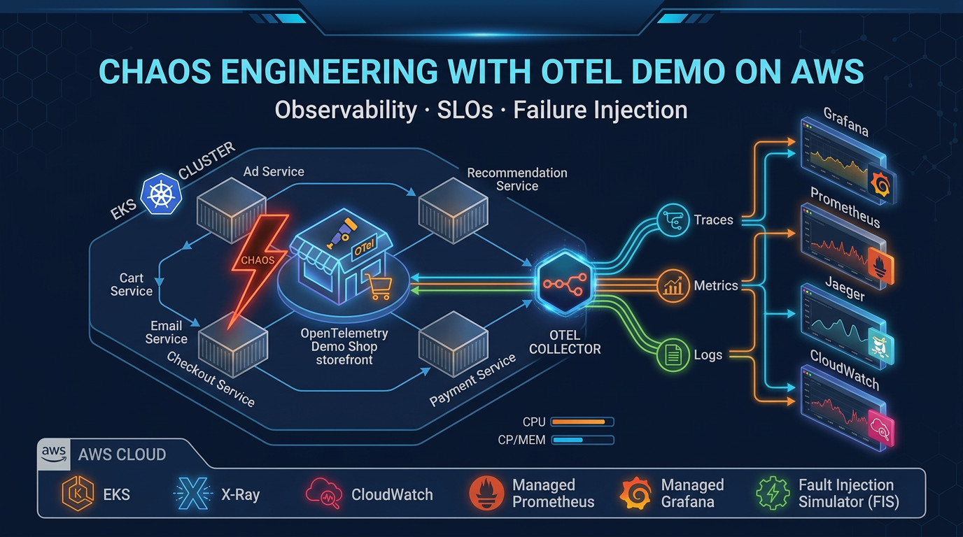
Table of Contents
Most observability training stops at “here’s what a metric looks like” and “here’s a trace waterfall.” That’s theory. You only learn observability when you’re under pressure—diagnosing a broken system with incomplete signals, messy dashboards, and no clear answers.
The AWS observability team built a game that forces exactly that situation.
OTel Demo: The Game is a chaos engineering sandbox that takes the official OpenTelemetry Demo (15 microservices, real distributed system) and injects 44 engineered failures across 12 categories. Your job: observe the degradation using metrics, traces, and logs, then submit your hypothesis about what broke. An LLM (Bedrock Nova Pro, by default) scores your answer. You remediate and move to the next round.
No Grafana. No Prometheus. No Jaeger. Pure AWS-native observability on EKS—CloudWatch, X-Ray, CloudWatch Logs—with an AI judge keeping score. It’s a deliberate statement about how to do observability at scale on AWS without adopting another monitoring vendor.
Here’s everything you need to know about it.
What Makes This Different From Other OTel Demos
Most OpenTelemetry demos are passive: you deploy microservices, watch telemetry flow, maybe query a dashboard. OTel Demo: The Game is active and adversarial. Scenarios are randomized. Failures compound in unexpected ways. Your hypothesis must match the actual injected fault—vague answers get scored as vague.
Three design choices stand out:
AWS-native only. CloudWatch Metrics (derived from trace spans), X-Ray (traces), CloudWatch Logs (logs). No third-party backends. This is intentional. AWS added native OTLP HTTP ingestion to CloudWatch and X-Ray a few years ago, but most OTel projects still default to Prometheus + Grafana because “that’s what everyone uses.” This game proves you don’t need to. Fewer moving parts. One set of AWS IAM permissions. One vendor bill.
The spanmetrics connector. Most teams instrument separately: one agent for traces, a different one for metrics (Prometheus, StatsD, whatever). The OpenTelemetry Spanmetrics Connector skips that redundancy. It watches trace spans as they flow through the collector and automatically derives RED metrics (Rate, Errors, Duration) from the trace data. You get metrics without a metrics scraper. This game demonstrates why it’s a game-changer for reducing instrumentation complexity.
LLM as judge. Bedrock Nova Pro (or Claude, or any OpenAI-compatible model) reads your free-text hypothesis and scores it against the actual fault. “Pod restarted on payment service” matches “pod kill on payment”; “high latency” matches “network delay added to cart service.” The LLM doesn’t just check answers—it learns from your explanations. This is what SRE looks like when AI assists the diagnosis, not replaces it.
Architecture: Three Layers
The game has a clean separation. Understanding each layer tells you how to build observability into your own EKS clusters.
Layer 1: The Demo (15 Microservices)
OpenTelemetry maintains an official demo application—a realistic e-commerce system with a frontend, payment processor, inventory service, recommendations engine, fraud detector, and 10 more services. Each service is pre-instrumented to emit OTLP traces, metrics, and logs.
The game deploys this Helm chart into the otel-demo Kubernetes namespace on EKS. Standard setup. Nothing special. Just 15 real services talking to each other, every request generating telemetry.
Layer 2: The Collector (OTLP Pipelines)
A single OpenTelemetry Collector pod in the same namespace receives all OTLP data from the microservices. It runs three pipelines:
Traces → X-Ray (via SigV4-signed OTLP HTTP exporter) Metrics → CloudWatch Metrics (via SigV4-signed OTLP HTTP exporter) Logs → CloudWatch Logs (to log group /otel/demo, stream otel-demo-services)
The collector batches data (10-second timeout, 500-item threshold) and adds metadata: cloud.provider=aws, service names, request IDs. It strips unnecessary noise (socket peer attributes) so your CloudWatch dashboards stay readable.
Authentication is keyless: the collector pod runs under an IRSA service account (IAM Roles for Service Accounts), annotated with an IAM role that grants PutMetricData, PutTraceSegments, PutLogEvents, and a few read permissions.
One unusual detail: the collector uses a Spanmetrics Connector to derive metrics from traces. Instead of the microservices also shipping metrics via Prometheus or StatsD, the collector watches spans as they pass through and calculates:
traces.span.metrics.calls— number of spans (request rate)traces.span.metrics.duration— span duration histogram (latency)traces.span.metrics.errors— span status code (error rate)
One pipeline, three signals. The game demonstrates this pattern to show that you can reduce instrumentation overhead by 30–50% if you’re willing to derive metrics from traces instead of maintaining separate metrics.
Layer 3: The Game App (SvelteKit)
A separate Kubernetes Deployment in the odtg namespace runs the game interface: a SvelteKit application (Svelte 5, TypeScript, Vite) with real-time metrics charts (Chart.js), trace visualization (D3), and interactive gameplay.
The game app makes direct Kubernetes API calls to control the demo:
- Scale a pod to zero (simulating a crash)
- Patch a deployment’s CPU limits down (simulating resource contention)
- Modify environment variables (toggling feature flags)
- Inject network delays into ConfigMaps that services read
It also queries CloudWatch Metrics, X-Ray Traces, CloudWatch Logs Insights, and AWS Cost Explorer to show you what you’re observing and what it costs to observe it.
The app’s IRSA service account has three sets of permissions:
- Kubernetes API access (get, list, watch, patch, delete on pods, deployments, statefulsets, configmaps)
- AWS CloudWatch (PutMetricData, GetMetricData, GetMetricStatistics)
- AWS Bedrock (InvokeModel for hypothesis scoring and hint generation)
It’s deployed with 100m CPU request / 512Mi RAM limit. No heavy lifting. The CloudWatch queries and Bedrock calls are the expensive operations, both managed by the game logic.
The Spanmetrics Pattern: Deriving RED From Traces
This deserves its own section because it’s the most powerful and least understood feature of the game.
Most teams instrument observability like this: application code → sends metrics to Prometheus (or CloudWatch) AND sends traces to Jaeger (or X-Ray). Two separate protocols, two separate data flows, two separate storage systems. If you want to correlate metrics and traces, you have to join them by request ID or timing, which is lossy.
OpenTelemetry’s spanmetrics connector does something smarter. It sits between your instrumented applications and your observability backend. As traces flow through the collector, it watches span creation and completion, then derives metrics from the span data:
- Span started and completed → 1 call counted
- Span status is ERROR → 1 error counted
- Span duration = latency measurement → percentile histogram updated
No separate metrics instrumentation needed. No Prometheus scraping. The tracing pipeline generates the metrics for free.
The game configures this to point at CloudWatch Metrics, so your RED dashboards in CloudWatch are auto-populated from traces. Request rate, error rate, latency p99 — all derived from the same instrumentation.
The catch: this only works if your trace coverage is 100% (or close to it). If you’re sampling 10% of traces to save costs, your metrics are 10% accurate. The game teaches you this the hard way: you’ll spot metric gaps that correspond exactly to the traces you dropped. Real production incidents often hide in the sampled-away traces.
44 Chaos Scenarios Across 12 Categories
Here’s where the game forces learning. Each round, the chaos engine randomly selects a scenario and injects a failure:
| Category | Example Scenarios |
|---|---|
| Pod termination | Kill payment service, kill 2 services simultaneously |
| Network faults | Inject 500ms latency on cart service, drop 5% of packets to shipping |
| Resource constraints | Drop CPU limit on frontend to 50m, exhaust memory on recommendation engine |
| Feature flags | Toggle recommendation service offline, disable caching in checkout |
| Multi-service faults | Simultaneously: kill checkout + delay payment + drop inventory connections |
| Service cascades | Cart calls payment → payment calls fraud detector; kill fraud detector, watch cascade |
| (6 more categories) | … |
Each fault has metadata: affected services, difficulty level, expected observable symptoms, and the actual root cause.
The gameplay loop:
- Idle state: view dashboard, read metrics/traces/logs from previous round
- Trigger chaos: one of 44 scenarios is selected and injected
- Degrade: response times spike, error rates rise, specific services show RED metric changes
- Diagnose: you query CloudWatch, X-Ray, CloudWatch Logs; look for correlations
- Hypothesize: you submit a free-text answer (“payment pod crashed after 30s”, “network delay on cart service”, etc.)
- Score: Bedrock Nova Pro reads your answer and scores it 0–100% based on accuracy and completeness
- Remediate: game reverses all chaos mutations automatically, or you can manually fix it
- Repeat: next scenario
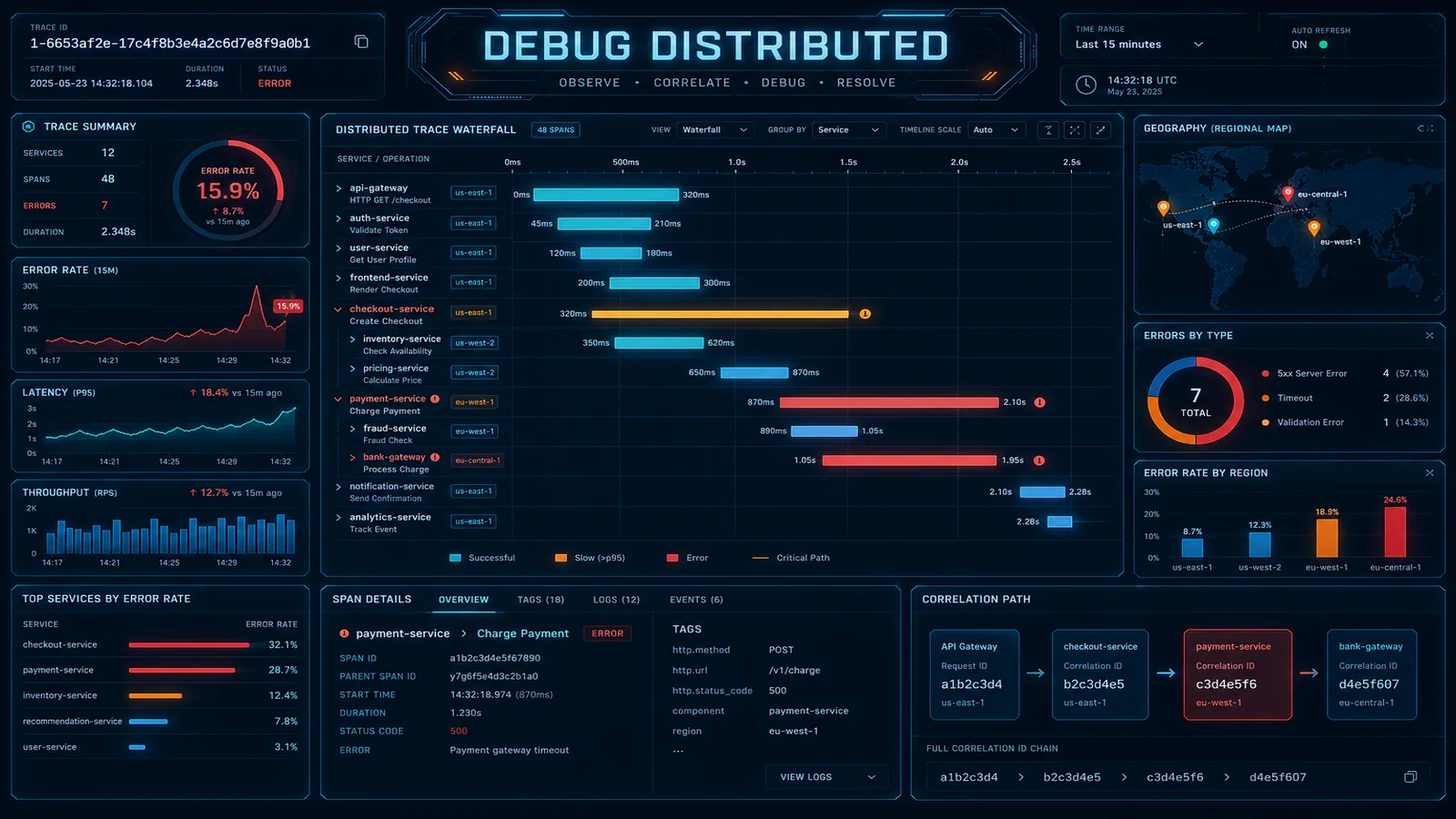
The gotcha: compound scenarios (two or three faults injected together) are almost impossible to diagnose from metrics alone. You need traces to see the causal chain. A pod restart with a simultaneous network delay looks like “everything is slow” in metrics; in traces, you see the requests timing out and retrying, which tells you something upstream is broken.
This teaches you why distributed tracing is not optional for production complexity.
LLM-Augmented Diagnosis: Bedrock as Your SRE Partner
The LLM scoring is the game’s most forward-looking feature. Instead of multiple choice answers (“Which of these broke?”), you submit a free-text hypothesis. Bedrock Nova Pro reads it, compares it to the actual injected fault, and assigns a score.
Example:
- You submit: “Payment service crashed because CPU went too high”
- Actual fault: Pod memory limit reduced to 256Mi, pod OOMKilled
- LLM assessment: “You identified the payment service and a resource constraint, but misidentified the resource type (CPU vs memory). Partial credit: 65%”
The LLM also provides hints on demand. Ask for help and it’ll say something like, “Check X-Ray for payment service errors in the last 5 minutes” or “Look at your container restart count in CloudWatch logs.”
This is a prototype for AI-assisted incident response. Instead of paging an on-call engineer who spends 15 minutes staring at dashboards, an LLM can quickly narrow the hypothesis space: “You see high latency; here are 5 scenarios to check first.”
Where this fails: LLM scoring only works if your hypothesis is grounded in observability data. If you guess randomly, the LLM will score you fairly but won’t help you improve. The game is teaching you to use observability to reason about failure, not to avoid it.
Secure Keyless AWS Access: IRSA and SigV4
The game demonstrates production-grade security for Kubernetes-to-AWS integration: IAM Roles for Service Accounts (IRSA) and SigV4 request signing.
Two service accounts are created:
- otel-collector: runs the OpenTelemetry Collector, has an IRSA role with CloudWatch Metrics, X-Ray, and CloudWatch Logs write permissions
- odtg: runs the game app, has an IRSA role with Kubernetes API, CloudWatch read, Cost Explorer, and Bedrock permissions
No long-lived IAM keys. No AWS_ACCESS_KEY_ID in ConfigMaps. No secrets in environment variables. Each pod gets a temporary, rotating STS token from the IRSA webhook, valid for 15 minutes.
The OTel Collector uses SigV4 to sign OTLP HTTP requests to CloudWatch and X-Ray endpoints. This is how AWS-native OTLP ingestion works: you don’t need an API key, just IAM permissions and request signing. Most docs still show API key examples (legacy), but production setups should always use SigV4 + IRSA.
This is the gold standard for Kubernetes-AWS integration. The game proves it works at scale.
Cost Observability: Seeing the Price Tag
Most observability platforms hide cost. Logs cost 5x less than traces, which cost 10x more than metrics—but you never see the breakdown. The game includes AWS Cost Explorer integration to show exactly what observability costs.
The dashboard displays:
- Total monthly cost for the demo infrastructure
- Cost breakdown: EKS cluster, RDS (if applicable), observability pipeline (CloudWatch ingestion, X-Ray traces, CloudWatch Logs)
- Per-service cost allocation using tags:
aws:eks:namespace,aws:eks:workload-name - Observability cost as % of total infrastructure cost
The gotcha: cost allocation tags must be activated in AWS Cost Explorer before they’re populated. Most teams miss this and can’t see per-pod costs until they go back and retroactively enable the tags. The game teaches you to think about cost observability as a first-class feature.
This is a lesson most commercial observability platforms avoid: if you knew what each service costs to observe, you might choose a different sampling strategy.
How to Deploy: Quick Start
Prerequisites:
- eksctl 0.170+ — EKS cluster creation
- Helm 3.x — Kubernetes package manager
- kubectl 1.28+ — Kubernetes CLI
- AWS CLI 2.x+ — AWS API access
- An AWS account with permissions for EKS, CloudWatch, X-Ray, Bedrock, Cost Explorer, IAM
Step 1: Create an EKS cluster
eksctl create cluster \
  --name otel-demo-cluster \
  --version 1.35 \
  --region eu-west-1 \
  --managed \
  --autos-scaling \
  --nodes 3
(The repo uses EKS Auto Mode, which manages node provisioning automatically. You can also specify manual node groups.)
Step 2: Install the OTel Demo via Helm
helm repo add open-telemetry https://open-telemetry.github.io/opentelemetry-helm-charts
helm install otel-demo open-telemetry/opentelemetry-demo \
  --namespace otel-demo \
  --create-namespace
Step 3: Deploy the game app
Clone the game repository, update values.yaml with your AWS region and Bedrock model choice, then:
helm install odtg ./game-helm-chart \
  --namespace odtg \
  --create-namespace
The game app will be accessible via an AWS ALB (Application Load Balancer) ingress. Grab the load balancer URL from your ingress:
kubectl get ingress -n odtgOpen it in your browser. You’re live.
Step 4 (Optional): Configure cost allocation
In the AWS Cost Explorer console, navigate to Cost Allocation Tags and activate the tags created by the deployment (aws:eks:namespace, aws:eks:workload-name, Project, Environment, CostCenter). Cost data will populate over the next 24 hours.
Full setup takes 15 minutes. Running costs: ~$100–200/month for an active cluster with observability pipeline.
When to Use This
Good fit:
- AWS workshops and internal training sessions
- SRE team onboarding (teaching junior engineers how observability works)
- Evaluating AWS-native observability vs. third-party stacks (Datadog, New Relic, Grafana Cloud)
- Understanding OpenTelemetry and chaos engineering hands-on
- Proof-of-concept for OTLP ingestion into CloudWatch + X-Ray
Not a fit:
- Production monitoring of your own applications (it’s a sandbox, not a platform)
- Replacing your existing observability vendor
- High-volume logging or metric ingestion (it’s a learning tool, not designed for scale)
Related Resources
If you’re deploying OpenTelemetry on AWS, these guides will deepen your understanding:
- How to Debug Production Issues Across Distributed AWS Systems — practical guide to using X-Ray and CloudWatch Logs Insights when chaos happens
- AWS CloudWatch Observability: Metrics, Logs, and Alarms Best Practices — deep dive on CloudWatch as your primary observability backend
- AWS CloudWatch Logging Costs: How to Avoid Logging Yourself Into Bankruptcy — cost management for CloudWatch Logs (directly relevant since the game tracks cost)
- Observability beyond CloudWatch (2026) — production ADOT topology, AMP/AMG, and Application Signals when you graduate from the game’s CloudWatch-only stack
- From One FIS Experiment to a Resilience Program (2026) — turning this hands-on tutorial into an organizational program: steady-state hypotheses, CloudWatch stop conditions, scheduled GameDays
- 10 AWS DevOps Practices We Actually Use in Production in 2026 — covers chaos engineering with AWS Fault Injection Simulator and observability integration
- How to Deploy EKS with Karpenter for Cost-Optimized Autoscaling — if you’re running this game repeatedly, Karpenter can manage scaling
- AWS Bedrock Nova Models: Performance, Cost, and When to Choose Over Claude — details on the LLM scoring engine
- AWS ECS vs EKS: Container Orchestration Decision Guide — context on why this game uses EKS vs. Fargate
Ready to Deploy Observability on AWS?
If your team is setting up AWS-native observability on EKS or wants to run OpenTelemetry in production without Grafana sprawl, we help teams go live with observability pipelines fast.
AWS Cloud Architect & AI Expert
AWS-certified cloud architect and AI expert with deep expertise in cloud migrations, cost optimization, and generative AI on AWS.