Bedrock Provisioned Throughput vs On-Demand: Break-Even Math for Production Workloads (2026)
Quick summary: Most teams buy Bedrock Provisioned Throughput too early or too late. This is the break-even math — by token volume, by model family, and by traffic shape — that we use in real FinOps engagements to decide which Bedrock pricing mode wins.
Key Takeaways
- Most teams buy Bedrock Provisioned Throughput too early or too late
- This is the break-even math — by token volume, by model family, and by traffic shape — that we use in real FinOps engagements to decide which Bedrock pricing mode wins
- The four Bedrock pricing modes, mapped Bedrock has four pricing modes that you can mix-and-match per model and per workload
- For deeper context on the model-selection and token-budget side of Bedrock cost, see our existing guide on Bedrock cost optimization, token budgets, and model selection
- How Provisioned Throughput is actually priced Bedrock Provisioned Throughput is sold in Model Units (MUs)
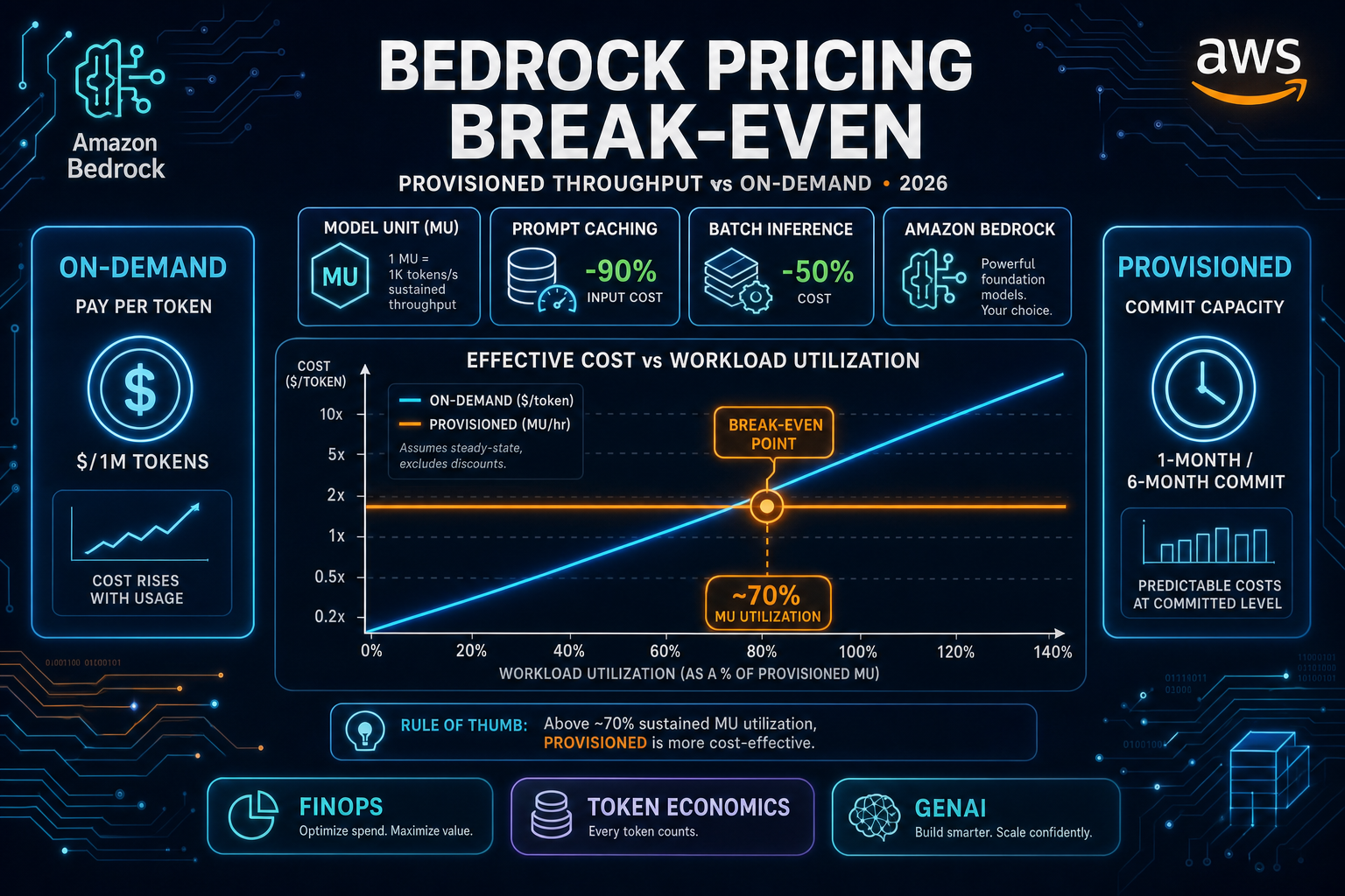
Table of Contents
Most engineering teams encounter Bedrock Provisioned Throughput in the same way: a finance review surfaces a Bedrock line item that has tripled month-over-month, someone screenshots the AWS pricing page, and a Slack thread starts about whether to “buy reserved capacity.”
The screenshot rarely contains enough information to make the decision. Provisioned Throughput is not a discount on on-demand pricing — it is a different pricing model with different units (Model Units per hour, not tokens), different commitment terms (1 month or 6 months, not pay-as-you-go), and a different break-even economics that depends heavily on traffic shape, not just total token volume.
This is the math we use in real FinOps engagements to decide whether a Bedrock workload should move to Provisioned Throughput, stay on on-demand, or apply the cheaper optimizations (Prompt Caching, Batch Inference) first.
The four Bedrock pricing modes, mapped
Bedrock has four pricing modes that you can mix-and-match per model and per workload. Each mode has a different cost shape — and the right answer for a given workload is usually a combination, not a single mode.
| Mode | What you pay for | Commitment | When it wins |
|---|---|---|---|
| On-Demand | Per input and output token, billed per request | None | Spiky traffic, dev/test, low total volume |
| Provisioned Throughput | Reserved Model Units (MUs) per hour | 1 month or 6 months | Sustained high-throughput steady-state traffic |
| Batch Inference | Per token, ~50% discount vs on-demand | None — async jobs only | Overnight or queued non-real-time workloads |
| Prompt Caching | Cached input tokens at ~10% of on-demand input rate | None | Long static prefixes reused across many requests |
The most common cost-optimization mistake we see is teams jumping straight to Provisioned Throughput because it sounds like a “reserved instance for AI.” Provisioned Throughput has the highest commitment and the longest payback time of the four modes. The cheaper optimizations should be exhausted first.
For deeper context on the model-selection and token-budget side of Bedrock cost, see our existing guide on Bedrock cost optimization, token budgets, and model selection.
How Provisioned Throughput is actually priced
Bedrock Provisioned Throughput is sold in Model Units (MUs). Each MU delivers a guaranteed minimum throughput — measured in input tokens per minute and output tokens per minute — for one specific foundation model.
The pricing has three dimensions:
- Hourly MU rate — Varies by model family. Smaller models (Haiku-class, Nova Micro/Lite) have lower hourly rates than larger models (Sonnet, Opus, Nova Pro/Premier).
- Commitment term —
No commitis the most expensive (and only available for some models).1-month commitis cheaper.6-month commitis the cheapest per-hour rate. - Number of MUs — You can provision multiple MUs of the same model in the same region for higher aggregate throughput. Capacity scales linearly; pricing scales linearly.
A single MU of a Claude Sonnet-class model on a 6-month commit can deliver tens of thousands of input tokens per minute — enough for most production applications below a few hundred concurrent users. A single MU of a Haiku-class model delivers materially more tokens per minute at a lower hourly rate, because the model is cheaper to serve.
Verify before committing. Per-MU hourly rates and per-MU throughput vary by model and change as AWS releases updated foundation model versions. The decision math below uses the ratio of provisioned-to-on-demand cost, which is more stable than any specific dollar figure. Always cross-check the current numbers on the Amazon Bedrock Pricing page before signing a 6-month commit.
The break-even formula
There are two equivalent ways to think about the break-even point. Pick whichever matches the data you actually have.
Formulation 1: Sustained tokens per minute
If you know your sustained throughput (input + output tokens per minute averaged across the hour), the break-even question is:
At what tokens-per-minute does the per-token economics of one MU undercut on-demand?
Let:
T_in= input tokens per minute delivered by one MUT_out= output tokens per minute delivered by one MUR_mu= MU hourly cost (commit-term-adjusted)R_in= on-demand input rate (per token)R_out= on-demand output rate (per token)
The hourly on-demand cost of producing the same throughput as one MU is:
hourly_on_demand_cost = (T_in × 60 × R_in) + (T_out × 60 × R_out)The break-even utilization is:
break_even_utilization = R_mu / hourly_on_demand_costIf your actual hourly utilization of one MU is above the break-even percentage, Provisioned Throughput is cheaper. Below, on-demand is cheaper.
For most current Claude and Nova model families on a 1-month commit, the break-even utilization tends to land between 60% and 75% of one MU’s full capacity — sustained, every hour of every day, for the entire commitment.
Formulation 2: Total tokens per month
If you only know your total monthly token volume (not the throughput shape), use:
break_even_monthly_tokens ≈ (R_mu × 730) / weighted_per_token_ratewhere weighted_per_token_rate is the average of input and output rates weighted by your actual input-to-output ratio. The 730 is the approximate hours in a month.
This formulation is less accurate than the throughput-based one because it ignores traffic shape — a workload that produces all its tokens in 4 hours per day will under-utilize Provisioned Throughput dramatically even if the monthly total looks high.
Reproduce this — The break-even calculator we use in engagements is open: clone
palpalani/bedrock-break-even-sheet, openbedrock-break-even.xlsx, and edit the Inputs sheet (model family, monthly input tokens, monthly output tokens, traffic shape, prompt-cache hit rate). The Recommendation sheet computes monthly on-demand, monthly batch, monthly provisioned (1-month and 6-month commits), effective utilization, and the call.make testruns the five scenarios below and asserts the recommendations match. Pricing constants live in one editable sheet — refresh them from the Bedrock pricing page before signing any commit.
Five worked scenarios
To make the math concrete, here are five typical workload shapes and the right call for each. The dollar figures are illustrative for the structure of the decision — the absolute amounts will move with model pricing, but the relative call is stable.
Scenario 1: Internal AI assistant, 12M tokens/month, business hours only
A SaaS company runs an internal Q&A assistant on Claude Haiku. Token volume is 12M/month, but it concentrates in a 9-hour business-hours window across a 5-day workweek. Effective active hours per month ≈ 195.
- On-demand monthly cost: 12M tokens × Haiku weighted rate
- One MU at the smallest commit term: still pays for 730 hours/month, of which only 195 are active
Call: Stay on-demand. Even though token volume is non-trivial, the traffic shape leaves the MU idle 73% of the time. Apply Prompt Caching to the static system prompt for further savings.
Scenario 2: Customer-facing chatbot — the math we ran for a real engagement
From a real engagement — A consumer fintech running a customer-facing chatbot on Claude Sonnet 4. Bedrock line item was $14,300/mo and trending up month-over-month. Traffic shape: steady around 80M tokens/month with a 2× peak-to-trough ratio across two geographies. We recommended provisioning one MU of Sonnet 4 on a 1-month commit for the steady traffic, leaving on-demand to absorb spikes, and enabling Prompt Caching on the system prompt and tool definitions. Thirty days later the Bedrock line item was $8,900/mo, a saving of $5,400/mo (~38%), with no degradation in p95 latency.
The math we ran for this engagement:
- On-demand monthly cost: ~80M × Sonnet weighted rate
- Throughput requirement at the 70th-percentile hour: roughly 110K tokens/hour
- One MU of Sonnet 4 (1-month commit) likely delivers more than that at full utilization
Call: Provision one MU of Sonnet 4 (1-month commit) for the steady traffic, leave on-demand to absorb the spikes. Re-evaluate at the next renewal — if utilization holds, move to a 6-month commit for the lower hourly rate.
Scenario 3: RAG-heavy enterprise search, 350M tokens/month, steady 24/7
A regulated enterprise running a Knowledge Base-backed search assistant on Claude Sonnet 4. Long retrieved-context inputs (input-heavy ratio), steady 24/7 throughput.
- The input-heavy ratio means weighted per-token rate is closer to the input rate than output rate
- Steady 24/7 means MU utilization can plausibly hit 80%+
- 350M tokens/month sustained is firmly in the territory where Provisioned Throughput wins
Call: Provision two MUs of Sonnet 4 on a 6-month commit. Apply Prompt Caching to the system prompt and the RAG retrieval template — this further reduces input-token cost on top of the provisioned discount. Use on-demand only as overflow.
Scenario 4: Overnight document processing, 200M tokens/month, all between 1am and 6am
A legal-tech platform that ingests case files and generates structured summaries. All inference is asynchronous and runs in a 5-hour overnight window.
- Provisioned Throughput utilization across 24 hours: ~21% — far below break-even
- On-demand for 200M tokens is expensive
- Batch Inference matches the workload shape exactly: async, non-real-time, can tolerate hours of latency
Call: Move to Bedrock Batch Inference. The ~50% per-token discount applies to the entire 200M monthly volume with zero capacity commitment. Provisioned Throughput would be wasted on this traffic shape; Batch is the correct primitive.
Scenario 5: Custom fine-tuned model, 30M tokens/month
A healthcare SaaS fine-tuned a Claude Haiku model on internal terminology. Total volume is modest at 30M tokens/month.
- Custom-imported and fine-tuned Bedrock models do not have an on-demand tier — they are served exclusively via Provisioned Throughput
- The decision is not “Provisioned vs on-demand” — it is “Provisioned, or do not use a custom model at all”
Call: Either provision the minimum MU for the custom model (and accept the 24/7 hourly cost as the floor), or step back and re-evaluate whether RAG against a base Claude Haiku on on-demand could deliver the required quality at a fraction of the cost. We have walked many teams off fine-tuning at this volume — the operational and cost burden of a permanent provisioned MU rarely pays back below ~100M tokens/month.
For more on this trade-off, see our guide on Bedrock as the fastest path to enterprise GenAI.
The order to apply optimizations
Provisioned Throughput should not be the first lever. The cost-optimization sequence we follow in real engagements:
- Right-size the model. Measure on-demand cost per use case at Haiku-class models first. Most workloads do not need Sonnet or Opus for 60–70% of their invocations. Model selection is a 5–20× cost lever; everything below is fractional in comparison.
- Trim the prompt. System prompts above 500 tokens are usually inflated. Cut redundant instructions and verbose role-play preambles.
- Enable Prompt Caching. For long static prefixes (system prompts, RAG context, agent orchestration scaffolds), cached input tokens are roughly 10% of the on-demand rate. Free to enable, near-zero risk.
- Move async work to Batch Inference. Anything that is not real-time user-facing — overnight summarization, document classification, embedding generation, scheduled reports — belongs in Batch.
- Then, and only then, evaluate Provisioned Throughput. Run the break-even math against your measured 70th-percentile-hour utilization, not your peak.
Steps 1–4 typically cut Bedrock spend by 40–70% before any commitment to Provisioned Throughput is on the table. We have seen teams sign 6-month Provisioned Throughput commits and then realize three weeks later that Prompt Caching alone would have made the commitment redundant.
Common mistakes when buying Provisioned Throughput
These are the patterns we see in cost reviews after a Provisioned Throughput commitment is already in place.
Provisioning for peak traffic. A workload with a 4× peak-to-trough ratio that provisions for peak utilizes the MU at 25% on average. The on-demand cost of the peak hours alone would have been cheaper than the wasted provisioned hours. Provision for the 70th-percentile-hour and let on-demand absorb the spikes.
Seen at: a retail SaaS running 1 MU of Sonnet 4 at ~18% Mon-Thu utilization; the same workload on on-demand would have been roughly 40% cheaper.
Ignoring the model-version refresh cycle. A 6-month commit on a model that gets superseded by a better, cheaper version after month 2 is a stranded asset. Anthropic and Amazon refresh model families on roughly 6–12 month cycles; commit terms longer than 1 month should be a deliberate bet on model stability, not a default.
Seen at: a media-tech engagement that signed 6 months of Sonnet 4 capacity three weeks before Sonnet 4.5 shipped.
Double-counting Bedrock Agents costs. Agent-orchestrated invocations are billed against the underlying model’s pricing mode. If the model is on Provisioned Throughput, the agent’s token consumption draws against the provisioned MU. If you separately budget for “Agent costs” on top of foundation-model costs, you are double-counting.
Seen at: a B2B logistics platform whose finance team had budgeted Bedrock Agents at ~$6k/mo on top of the underlying Sonnet provisioned spend; the actual incremental cost was zero.
Underestimating Knowledge Base baseline cost. Bedrock Knowledge Base on the OpenSearch Serverless backing store has a 2-OCU minimum at $0.24/OCU-hour — about $345/month before a single query runs. This is independent of whether the foundation model is on-demand or Provisioned Throughput. For low-query workloads under 10K queries/month, evaluate Aurora PostgreSQL with pgvector as a lower-floor alternative.
Seen at: a healthcare RAG pilot with ~3,200 queries/month — the effective per-query cost was over $0.10 before the model invocation, dominated by the OpenSearch Serverless floor.
Forgetting cross-region inference profiles. Cross-region inference profiles can change the effective per-token economics for some models because they unlock capacity that a single-region on-demand call would have throttled. Run the on-demand baseline with inference profiles enabled before assuming you need Provisioned Throughput for capacity reasons.
Seen at: a fintech batch-classification workload that was about to commit to 2 MUs purely for capacity reasons — enabling cross-region inference profiles eliminated the throttling and made the on-demand baseline viable.
Multi-region Provisioned Throughput
Provisioned Throughput is purchased per region. Workloads with users distributed across geographies face a choice:
- Single-region provisioned, cross-region inference profiles for the rest — Provision in your primary region; let inference profiles route excess traffic to other regions on on-demand pricing. This is the cheapest setup for most workloads with a clear primary region.
- Multi-region provisioned with regional load balancing — Provision in two or three regions for genuine multi-region active-active. Adds operational complexity (capacity management per region) and ties up commitment in regions that may be lower-utilized. Worth it only when latency or data-residency requirements force per-region capacity.
- One region only, accept latency — For internal tools or non-latency-sensitive workloads, single-region Provisioned Throughput with no failover is operationally simplest. Document the failure mode in your runbook.
Treat multi-region provisioned throughput the same way you would treat multi-region RDS: only buy it when there is a real availability or latency requirement that single-region with failover cannot meet. Multi-region is rarely the cheapest answer.
Measuring before you commit
Before signing any Provisioned Throughput commitment, run a 14-day on-demand measurement. The data you need:
InvocationCountper model per hour — From CloudWatch Bedrock metrics, partitioned by model IDInputTokenCountandOutputTokenCountper hour — Same dimensions- Per-hour utilization curve —
(InputTokenCount × 60s + OutputTokenCount × 60s) / one_MU_throughput
The CLI you can run today against your own account, replacing the model ID with the one you are evaluating:
# Hourly input-token sums for the last 14 days, single model.
aws cloudwatch get-metric-statistics \
  --namespace AWS/Bedrock \
  --metric-name InputTokenCount \
  --dimensions Name=ModelId,Value=anthropic.claude-sonnet-4-v1:0 \
  --start-time "$(date -u -v-14d +%Y-%m-%dT%H:%M:%SZ)" \
  --end-time   "$(date -u +%Y-%m-%dT%H:%M:%SZ)" \
  --period 3600 \
  --statistics Sum \
  --region us-east-1 \
  > input-tokens-14d.json

# Same for OutputTokenCount and InvocationCount.
aws cloudwatch get-metric-statistics --namespace AWS/Bedrock --metric-name OutputTokenCount  \
  --dimensions Name=ModelId,Value=anthropic.claude-sonnet-4-v1:0 \
  --start-time "$(date -u -v-14d +%Y-%m-%dT%H:%M:%SZ)" --end-time "$(date -u +%Y-%m-%dT%H:%M:%SZ)" \
  --period 3600 --statistics Sum --region us-east-1 > output-tokens-14d.json
Then compute the 95th-percentile sustained tokens-per-minute with jq:
jq -r '.Datapoints | sort_by(.Timestamp) | .[].Sum' input-tokens-14d.json \
  | awk '{print $1/60}' \
  | sort -n \
  | awk 'BEGIN{c=0} {a[c++]=$1} END{print a[int(c*0.95)]}'
The output is the input-tokens-per-minute rate sustained across the 95th-percentile hour of the last two weeks. Compare that to the per-MU T_in for your candidate model from the Bedrock pricing page — that ratio is your projected MU utilization. The same shape works for OutputTokenCount.
macOS users — replace
date -u -v-14dwithdate -u -d '14 days ago'on Linux. Both produce ISO-8601 UTC. Ifawknumerics surprise you on locale-specific systems, prependLC_ALL=C.
Plot the per-hour utilization across the 14 days. Look at:
- Median hour — If the median is below 50%, Provisioned Throughput is unlikely to win even on a 6-month commit.
- 70th-percentile hour — This is the right size to provision. Above this, on-demand handles the spikes.
- Peak hour — Used for capacity planning, not for sizing the commitment.
This 14-day exercise also surfaces the data you need for the cheaper optimizations:
- Hours with high prefix-overlap rate are Prompt Caching candidates
- Hours dominated by asynchronous batch jobs are Batch Inference candidates
- Hours where one model is invoked at high volume but a smaller model would have sufficed are model-selection candidates
We run this measurement as part of every Cloud Cost Optimization engagement that touches GenAI workloads. The output is a single dashboard that surfaces which optimization to apply in which hour-block.
What we got wrong — A media analytics SaaS hit every condition in the break-even formula. Sustained 24/7 throughput, ~78% projected MU utilization on Sonnet, the math was unambiguous. We recommended a 6-month commit on 2 MUs of Sonnet 4 against ~280M tokens/month. Six weeks in, Anthropic shipped Sonnet 4.5 with materially better quality at a lower per-token rate, and the team’s product roadmap shifted from a synchronous chat feature to a batch-style overnight workflow. The commit had 4 months and roughly $19,000 of stranded capacity remaining. The fix going forward: default to 1-month commits unless the customer has an explicit “no model upgrades for 6 months” policy, and re-validate the traffic-shape assumption two weeks post-launch before committing beyond month one. The formula was right; the input assumptions had a half-life we underestimated.
When Provisioned Throughput is the right call
To summarize, Provisioned Throughput is the right answer when all of these are true:
- Steady-state traffic that sustains 60%+ of one MU’s capacity for the majority of hours
- A 1-month or 6-month commitment is acceptable given your model-refresh tolerance
- The cheaper optimizations (right-sizing the model, trimming prompts, Prompt Caching, Batch Inference) have been applied or are not applicable
- The workload uses a custom-imported or fine-tuned model (in which case the choice is forced)
Below those bars, on-demand plus the cheaper optimizations is almost always the right answer. The most common pattern at scale is Provisioned Throughput for the predictable steady-state, on-demand for the spikes, Batch for the async work, and Prompt Caching applied across all of the above — not one mode picked exclusively.
If You Only Do One Thing This Quarter
Turn on Prompt Caching for your three highest-volume Bedrock prompts before evaluating Provisioned Throughput. Median observed savings on input-token cost across the workloads we have measured: 35–60% for prompts with stable system instructions or RAG retrieval scaffolds. Time to implement: roughly two hours per prompt — change the request payload to mark the cacheable prefix (Anthropic models support cache_control on Bedrock invocations) and re-deploy.
Two reasons this is the highest-ROI single move:
- Free to enable, near-zero risk. No commitment, no capacity reservation, no model change. If it does not help your prompt shape, the bill is unchanged.
- It changes the inputs to the break-even formula. Caching reduces the effective input-token cost on cached hours by ~90%, which pushes the on-demand baseline lower — and therefore raises the throughput threshold at which Provisioned Throughput wins. Multiple teams we have worked with concluded “we need PT” pre-caching and “we don’t” post-caching, three weeks apart.
If you are already caching aggressively and the bill is still climbing, then run the 14-day measurement above, then open the calculator, then size a 1-month commit. In that order.
What about Claude Platform on AWS?
While this post was being written, AWS announced Claude Platform on AWS — a new path that delivers Anthropic’s native Claude experience billed and authenticated through your AWS account. IAM handles access, billing rolls into your existing AWS invoice, and CloudTrail logs every call. There is no separate Anthropic account or API key.
The early reaction in the engineering community captures the appeal honestly. As one practitioner put it: “Bedrock is fine but it always felt like one layer too many when all you want is Claude with decent enterprise controls.” The simplification argument is real — for teams that wanted Claude on AWS billing without Bedrock’s wrapper, this is a more direct path.
But the official AWS page is explicit about the trade-off: customer data on Claude Platform is processed by Anthropic outside the AWS boundary. Bedrock keeps data within AWS infrastructure; Claude Platform does not. For regulated workloads — HIPAA-eligible healthcare, PCI cardholder data, FedRAMP environments, EU data-residency obligations — that single line moves the decision back to Bedrock unconditionally. The Provisioned Throughput math in this guide still applies; the alternative path simply is not available for those workloads.
For non-residency-constrained workloads (internal productivity tools, public marketing copy generation, R&D), Claude Platform on AWS may turn out to be the simpler operational answer once pricing is published. As of writing, the page lists the service as “Coming Soon” with no pricing details — so any direct cost comparison is premature. We will update this post when pricing and regional availability are announced.
The practical effect of the announcement on the Provisioned Throughput decision is to sharpen it, not weaken it: if you have already concluded that data-residency forces you onto Bedrock, the only remaining question is whether your sustained traffic justifies a commitment. That is the math this post is here to answer.
Where this fits in your AWS cost program
Bedrock is rarely the largest line item on an AWS bill — but it is the fastest-growing one across our portfolio in 2026, and the one most likely to surprise finance leaders quarter-over-quarter. The teams that handle this well treat Bedrock cost the same way they treat compute and database cost: with a measured baseline, an explicit optimization sequence, and commitments sized to the 70th-percentile-hour rather than the peak.
If you are at the point of evaluating Provisioned Throughput, you are in the territory where a structured FinOps review usually pays back inside the first month. Our Cloud Cost Optimization and Bedrock consulting engagements include this measurement and the resulting commitment plan. If you would rather work the numbers yourself, the AWS Bedrock Token Cost Calculator is a starting point — and the existing Bedrock cost optimization guide covers the optimization levers that come before any commitment.
AWS Cloud Architect & AI Expert
AWS-certified cloud architect and AI expert with deep expertise in cloud migrations, cost optimization, and generative AI on AWS.